Research Overview
An overview of my work at the Semeter Lab at Boston University.
1 Algorithms
1.1 Data Processing
1.1.1 Ionospheric Assumption Validation
For speed of computation, we use fast 2d and 3d natural neighbors interpolation (thick large-scale structures) and VISTA (thick medium-scale structures) (Video Imputation with SoftImpute, Temporal smoothing and Auxiliary data) to validate the ionospheric assumption.
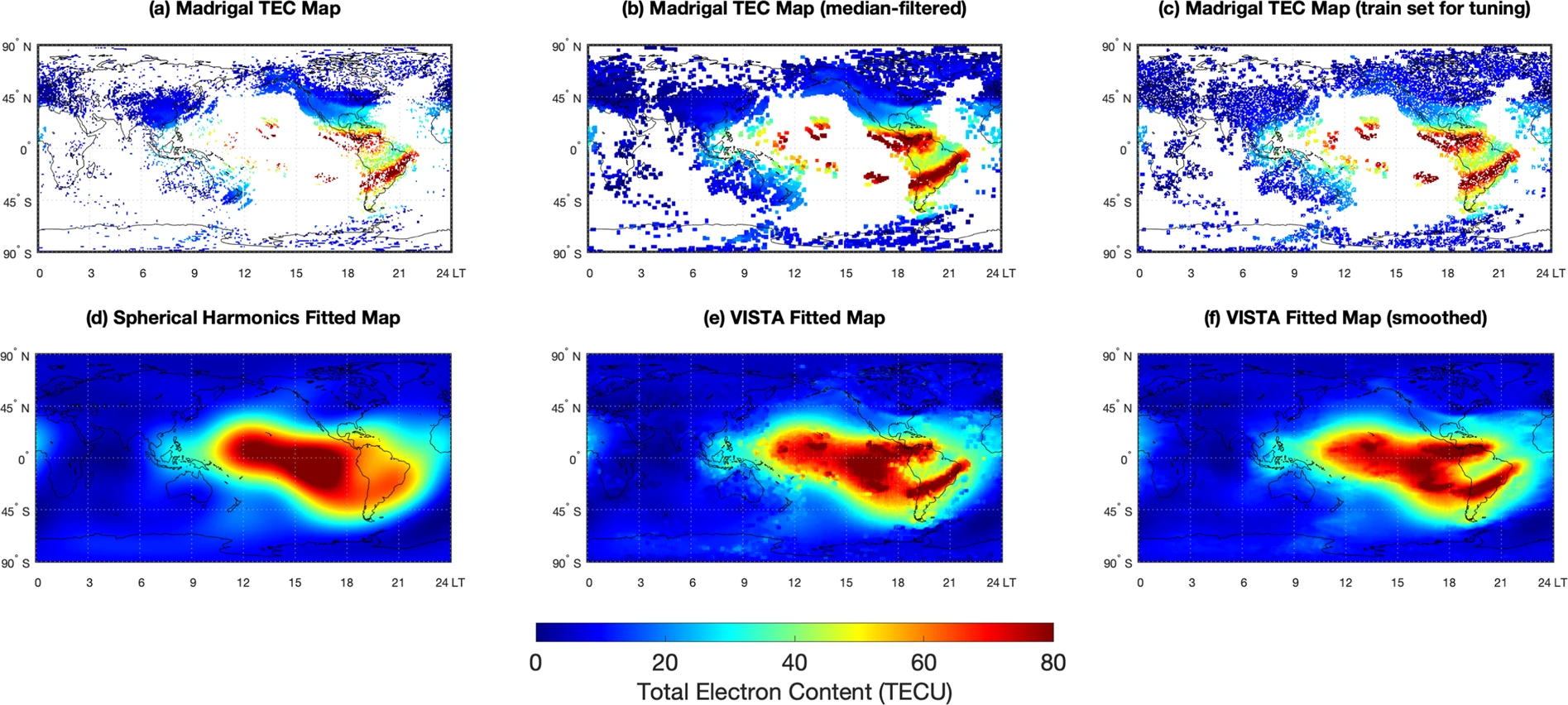
The assumption is (somewhat) invalid during solar storms, geophysical storms, magnetic reconnection with solar winds, coronal mass ejections, and so on.
1.1.2 RINEX conversion
Developed an internal Python package named rinexpy - looking to merge with georinex:
rinexpy Operations:
Merging and Editing RINEX Files: Provides the ability to merge multiple RINEX files into a single output. Allows for editing of the file contents, such as adjusting header information, modifying observation types, and managing data intervals.
Clock Jump Correction: Automatically detects and corrects clock jumps in GNSS observation data.
Ionospheric Correction: Applies higher-order ionospheric corrections to the GNSS data.
File Format Conversion: Supports converting BINEX and RTCM files into the RINEX format.
Interactive RINEX File Viewer: Includes an interactive, web-based viewer for RINEX files.
1.1.3 Analysis
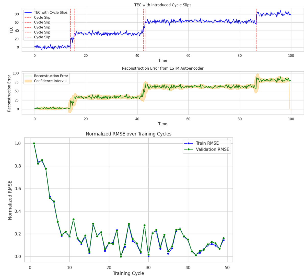
Cycle slip correction: We design machine learning models for cycle slip correction. These are better than the heuristic ‘stiching’ process that may remove important TEC jumps that could identify an ionospheric phenomenon.
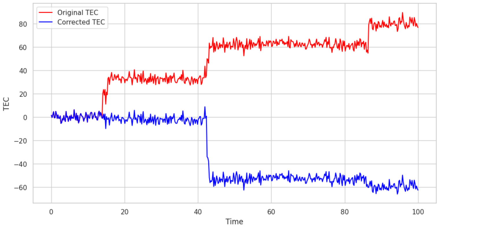
The technique used is LSTM-based autoencoders, for several reasons:
- The Poker Flat setups are the same receiver in roughly the same area, so we are justified in using LSTM-based autoencoders for this.
- Under the assumptions that the internals of Pixel phones suffer roughly the same wear-and-tear, autoencoders are straightforward to deploy on Sagemaker and call for inference.
We also account for multipath noise, temperature noise (Rideout and Coster), propagation errors, ionospheric delays, and utilize precise point positioning to estimate slant TEC as accurately as possible.
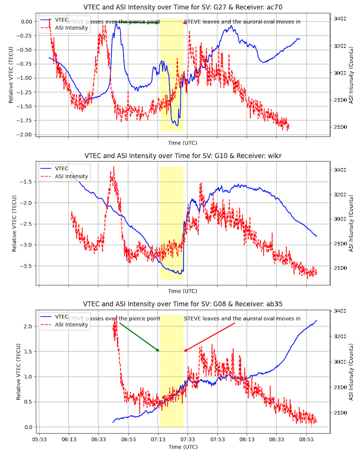
Time-series classification: How does TEC change during an auroral event?
Given a dataset of time-series TEC curves at some frequencies, we want to classify them to make an early-warning system for auroral events (so citizen scientists can go out and take photographs!)
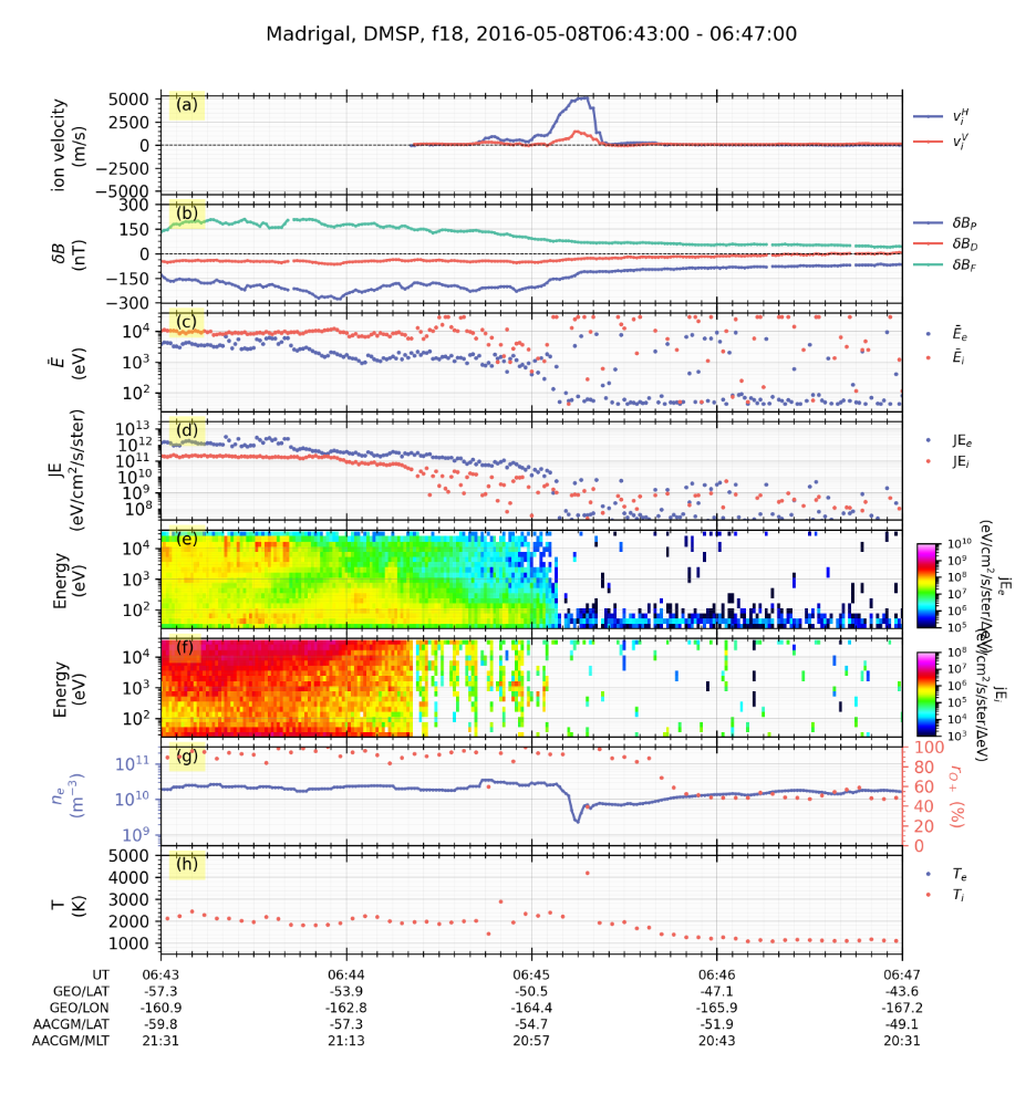
You can probe ionospheric conditions (such as from DMSP) and get extra time series:
Method for auroral phenomenon identification:
- Use 1D CNN to classify raw TEC changes as STEVE, SAPS, SAID, Discrete Aurora, Continuous Aurora, etc.
- Analyze satellite flyby data to see what ionospheric, magnetospheric, and thermospheric parameters change in that time period.
2 Computer Vision Algorithms
We use Max-Tree for faint phenomenon identification, active learning, monocular depth estimation (Depth Prediction Transformers), and Open Set recognition to identify STEVE in citizen science images.
The clustering model developed was to classify all-sky images of aurora - using ResNet-18 to extract features, used PCA to reduce dimensionality, and K-Means++ to cluster. Achieved silhouette score of 0.7, Davies-Bouldin index of 0.9, Calinski-Harabase index of 256 indicating high-quality cluster separation.
3 Life on Mars
Generated TEC maps from MARSIS data by modeling with two-layer Chapman functions for Martian ionosphere. Used VISTA to reconstruct (in 3D), 3d volumes of maps. Auxiliary guess was made using natural pixel decomposition, where the 3d structure estimated with tomography. Specifically, it is modeled as a Fredkin integral of the first kind and pLogMART is used as the matrix inversion algorithm. Simulated GPS propagation through it.